Explaining RNNs without neural networks

Terence Parr
Terence is a tech lead at Google and ex-Professor of computer/data science in University of San Francisco's MS in Data Science program and you might know him as the creator of the ANTLR parser generator.

Vanilla recurrent neural networks (RNNs) form the basis of more sophisticated models, such as LSTMs and GRUs. There are lots of great articles, books, and videos that describe the functionality, mathematics, and behavior of RNNs so, don't worry, this isn't yet another rehash. (See below for a list of resources.) My goal is to present an explanation that avoids the neural network metaphor, stripping it down to its essence—a series of vector transformations that result in embeddings for variable-length input vectors.

My learning style involves pounding away at something until I'm able to re-create it myself from fundamental components. This helps me to understand exactly what a model is doing and why it is doing it. You can ignore this article if you're familiar with standard neural network layers and are comfortable with RNN explanations that use them as building blocks. Since I'm still learning the details of neural networks, I wanted to (1) peer through those layers to the matrices and vectors beneath and (2) investigate the details of the training process. My starting point was Karpathy's RNN code snippet associated with The Unreasonable Effectiveness of Recurrent Neural Networks and then I absorbed details from Chapter 12 from Jeremy Howard's / Sylvain Gugger's book Deep Learning for Coders with fastai and PyTorch and Chapter 12 from Andrew Trask's Grokking Deep Learning.

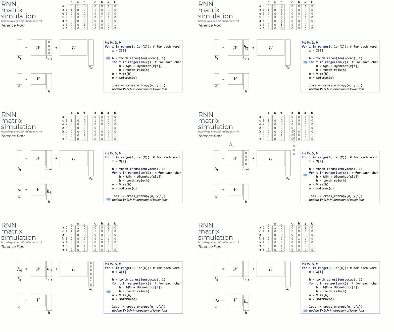
In this article, I hope to contribute a simple and visually-focused data-transformation perspective on RNNs using a trivial data set that maps words for "cat" to the associated natural language. The animation on the right was taken (and speeded up) from a youtube clip I made for this article. For my actual PyTorch-based implementations, I've provided notebooks that use a nontrivial family name to natural language data set. These links open my full implementation notebooks at colab:

• SGD (parameters updated after each record)
• minibatch (parameters updated after a small batch of records)
• vectorized minibatch (convert for-loop into matrix multiply)
• vectorized minibatch running on a GPU (use PyTorch to compute on GPU)

Table of contents

• 1. An RNN built with matrices and trained with SGD
  • The goal: meaningful vectors representing words
  • Encoding words as integers
  • Aggregating character vectors to encode words
  • Encoding and aggregating character vectors through matrix transforms
  • Learning the RNN matrices by training a classifier
• 2 Training an RNN with vectorized minibatch SGD
  • Computing loss using more than one input record
  • Converting the batch loop to vector operations
    • Processing batches, one character position at a time
    • Padding short words with 0 vectors on the left

Implementation Details and Concepts I learned

• What exactly is h (sometimes called s) in the recurrence relation representing an RNN: (leaving off the nonlinearity)? The variable name h is typically used because it represents the hidden state of the RNN. An RNN takes a variable-length input record of symbols (e.g., stock price sequence, document, sentence, or word) and generates a fixed-length vector in high dimensional space, called an embedding, that somehow meaningfully represents or encodes the input record. The vector is only associated with a single input record and is only meaningful in the context of a classification or regression problem; the RNN is just a component of a surrounding model. For example, the h vector is often passed through a final linear layer V (multiclass logistic regressor) to get model predictions.
• Does h contain learned parameters of the model? No. Vector h is a local variable holding the partial result as we process symbols of a single record but becomes the final embedding vector after the RNN processes the final input symbol. This vector is not updated as part of the gradient descent process; it is computed using the recurrence relation given above.
• Is h the RNN output? I think it depends on your perspective. Yes, that embedding vector comes out of the RNN and becomes the input to following layers, but it's definitely not the output of the entire model. The model output comes from, say, the application of another matrix, V to h.
• What is t and does it represent time? If your variable-length input record is a timeseries like sensor or stock quote data, then yes t represents time. Variable t is really just the iterator variable used by the RNN to step through the symbols of a single input record.
• What is backpropagation through time (BPTT)? BPTT is stochastic gradient descent (SGD) as applied to the specific case of RNNs that often process timeseries data. Backpropagation by itself means updating the parameters of the model in the direction of lower loss. BPTT refers to the case where we perform BP on m layers that reuse the same W and U for m symbols in the input record.
• Then what's truncated backpropagation or truncated BPTT? (First, let me point out that we don't need truncated BPTT for fairly short input records, such as we have for family names; my examples do not need to worry about truncated BPTT.) For large input records, such as documents, gradients across all (unrolled) RNN layers become expensive to compute and tend to vanish or explode, depending on our nonlinear activation function. To overcome this problem, we can simply stop the BP process after a certain number of gradient computations in the computation graph. It means not being able to update the model parameters based upon input symbols much earlier in the input stream. I sometimes see the length of the truncated window represented with variable bptt in code, which is pretty confusing. Note that h is still computed using the full computation as described by the recurrence relation. Truncated BP simply refers to how much information we use from BP to update the parameter models in W and U (and usually V). Vector h uses W and U but is not updated by BP. Model LMModel3 and Section "Maintaining the State of an RNN" of Chapter 12 in the fastai book explain this in detail.
• Each variable h is associated with a single input record and is initialized to the zero vector at the start of the associated record.
• Matrices W, U, V are initialized exactly once: before training begins.
• Matrices W, U, V are updated as part of the SGD process after the h embedding vector has been computed for each input record in the batch (or single word if using pure SGD). As we iterate through the symbols in time, the W, U, V matrices do not change, unless we are using truncated BPTT for very long input records.
• Minibatching is a small subset of the input records split between records, leaving all input records intact. However, in the situation where the input records are very big, minibatching can even involve splitting individual records, rather than just between records. Each record in a minibatch requires a separate h vector, leading to matrix H in my examples.
• When combining one-hot vectors for minibatching purposes, we must pad on the left not the right to avoid changing the computation. See this section: Padding short words with 0 vectors on the left.

Resources

• To get started with RNNs, I think the best first stop is probably MIT's RNN intro video to get an overview.
• Karpathy's well-known RNN blog and associated code snippet are really motivating and I used them as a basis to understand how the vectors flow through the RNN recurrence relation.
• Chapter 12 from Jeremy Howard's and Sylvain Gugger's book Deep Learning for Coders with fastai and PyTorch is chock-full of both high-level and low-level details. The other chapters are well worth reading too.
• Chapters 11 and 12 from Andrew Trask's Grokking Deep Learning has a lot of good stuff on word vectors and RNNs.
• Section 6.2 in François Chollet's Deep Learning with Python book does a really nice discussion and implementation using neural network layers; the book is very clearly written. It does, however, focus on keras whereas I'm using PyTorch for tensors in this article.
• Yannet Interian has a good notebook for training RNNs that map family names to languages.

Acknowledgements